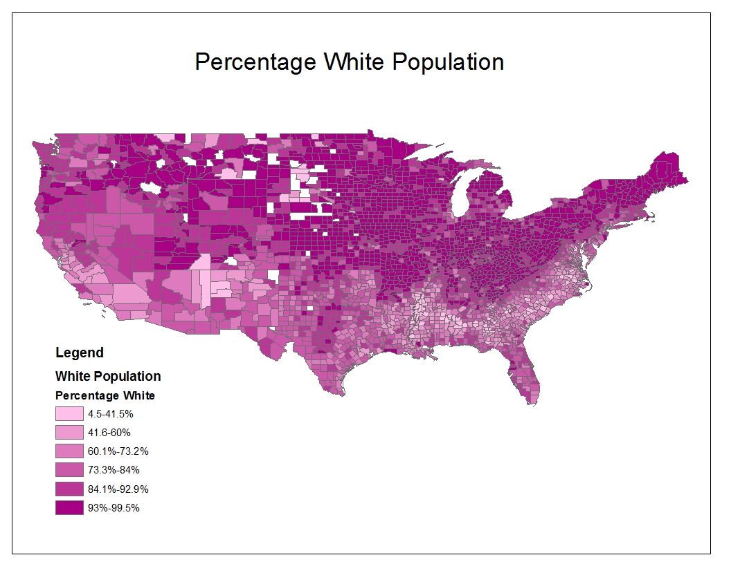
Total Pageviews

Wednesday, December 8, 2010

Lab 8: Census 2000-2010

White Population
Black Population


Asian Population
The above maps were created using 2000 Census Data and the population percentages of White, Black, and Asian populations by US County.  This was quite a frustrating project as I had some technical difficulties with ArcGIS, but I think the final product turned out fairly well. 

The White population across the United States is fairly self-explanatory.  The majority of the US population is white, so the percentages are quite high everywhere.  The most noticeable aspects of this map are the places that are less than 40%.  These areas are concentrated in the Four Corners area, probably due to Native American or Hispanic populations, as well as in the Southern United States where the Black population is quite high.  There are several places that are above 93% White, especially in the North, Midwest, and Northeastern US.  There are also areas that are blank, which I assume means that there is either no data available, or that there is no significant population in those areas.  

The Black population is quite concentrated.  Across most of the US there is less than 4%, and the high concentrations lie in the Southern US.  This is where slavery was last abolished, and therefore the African American population is quite high. 

The Asian population in the United States is most concentrated on the West Coast.  There are also some concentrations on the Northern East Coast.  Most of the country has less than 5% Asian populations, but some places on the East Coast have us to 46%.  This is because the Asians historically have migrated to these areas, and there are established ethnic enclaves. 

This Census map series was both helpful in mastery of ArcGIS, and informative about the US population.  I find it exciting that I have access to this data, and on campus I have access to this program.  Being able to make my own map of Census data has been rewarding.  GIS seems like an exciting and growing field with enormous potential.  Although there are pitfalls with popular access to such tools, there are far more opportunities for education and analysis.  The applications are vast and the implications are huge. 

Tuesday, November 23, 2010

Lab 7: Mapping the Station Fire in Arc GIS

Today I will be analyzing the LA County Station Fire of 2009.   This fire began August 26th 2009, and ended October 16th 2009.  It began in the Angeles National Forest, destroyed over 89 home, and killed two firefighters.   It was the largest fire in the modern history of LA County, burning over 160,000 acres. 

Below are maps that I have created to trace the spread patterns across area and elevation.  As you can see, the fire spread "up-hill," and into the higher elevation regions.  If you scroll down, I will discuss the spread of each map. 


Reference Map

Fire Perimeter with Elevation


Fire Stage 1: 5205 Acres
 This first stage of the fire was started by arson.  Accelerant was discovered at the scene.
Fire Stage 2: 13,891 Acres
 After only a few hours, the fire had more than doubled in area.  At this point, a pattern is difficult to discern, but the spread is to the east and west for the most part.
Fire Stage 3: 35,881 Acres
 Close to 24 hours after the start of the fire, you can see that the fire is spreading to the higher elevation areas, and now in a northern direction.  This winds must have shifted at this point. 
Fire Stage 4: 115,575 Acres
 The next day, the fire pattern spread along the hills to the east and west of the previous burn pattern.  Again, the fire seems to be move faster "up-hill."
Fire Stage 5: 136,246 Acres
The final map that I have posted spans most of the major damage of the Station Fire.  As you can see, not just elevation had an effect on the burn pattern, but the fire did seem to spread more in the higher elevation areas.  From the original spot, the spread is to the north, and somewhat to the east and west.  Infrequently did the fire move to lower elevations, or to the south.  Fire moves faster and more intensely uphill than down, and the steeper the slope the faster they move.  Wind also tends to flow uphill, which helps the fire spread. 

According to my findings, locations uphill of a fire source are much more at risk than those that are downhill.  Predictions about spread can also be made by studying the wind patterns.  Subsequently, it would make sense to concentrate fire prevention resources near areas with other risk facts combined with a quick increase in slope.  Structures and homes built in this area are at high risk. 


Bibliography

"2009 California Wildfires." Wikipedia, the Free Encyclopedia. 1 Nov. 2010. Web. 23 Nov. 2010. <http://en.wikipedia.org/wiki/Station_Fire_(2009)#Los_Angeles_County>.
"All Station Fire Perimeters." Los Angeles County Enterprise GIS. Los Angeles County, 2 Sept. 2009. Web. 23 Nov. 2010. <http://gis.lacounty.gov/eGIS/?cat=11>.
"Digital Elevation Model." Seamless Data Warehouse. U.S. Geological Survey, 30 Sept. 2010. Web. 23 Nov. 2010. <http://seamless.usgs.gov/>.
"Facts About Fire." Ontario Ministry of Natural Resources. Ontario Ministry of Natural Resources, 5 June 2009. Web. 23 Nov. 2010. <http://www.mnr.gov.on.ca/en/Business/AFFM/2ColumnSubPage/STEL02_165825.html>.

 "HowStuffWorks "Topography and Wildfires"" Howstuffworks "Science" Web. 23 Nov. 2010. <http://science.howstuffworks.com/nature/natural-disasters/wildfire3.htm>.


Friday, November 19, 2010

Lab 6: DEMs in ArcGis

This data is taken from a location in Eastern Arizona.  I chose it because of the interesting changes in elevation.  There are drastic changes in elevation which I believe to be the edges of plateaus.  This was a very interesting lab because I got to work on my own to create models, which I never thought possible.  It's great that students like myself can just access this type of data to work with and manipulate for the purposes of learning!

Spatial Reference:  GCS North American 1983-
Raster:  ned_34737954
Datum: D_North_American_1983

Extent:
left: -112.26
right: -111.68
top: 35.17
bottom: 34.84

Digital Elevation Model with Hillshade


Slope 


Aspect


3-D Model

Friday, November 12, 2010

Lab 5: Projections in ArcGis

Conformal

  • Mercator Projection: 10,148 Miles between Washington, D.C. and
    Kabul, Afghanistan


  • Gall Stereographic:   7,985 Miles between Washington, D.C. and
    Kabul, Afghanistan
Equal Area:

  • Sinusoidal:  8,113 Miles between Washington, D.C. and
    Kabul, Afghanistan
  • Bonne: 6,707 Miles between Washington, D.C. and
    Kabul, Afghanistan

Equidistant:

  • Equidistant Conic: 6,981 Miles between Washington, D.C. and
    Kabul, Afghanistan
  • Equidistant Cylindrical: 5,101 Miles between Washington, D.C. and
    Kabul, Afghanistan
               These maps were created to display different features.  The Conformal Maps preserve angles locally.  The Equal Area Maps preserve area, and the Equidistant Maps preserve distance.  As you can see by the distances listed, the differing projections provide contrasting information.  The Conformal Maps have very skewed area, as well as distance, the Equal Area Maps have skewed angles and distances, and the Equidistant Maps have skewed angles and areas.  They each have their purposes, advantages, and disadvantages. 
              The significance of being able to create these varying maps is huge.  For purposes of navigation, measurement, and perception, each map creates an opportunity to have a portable "globe" in one's pocket, depending on their purpose and needs. These projections all serve their own purpose, and are incredibly useful.  
               There are perils associated with various map projections.  This can be seen just by looking at the differences in the distance between Washington, D.C. and Kabul, Afghanistan.  If the wrong map is used for, lets say, launching a missile, then the missile could miss it's target my hundreds of miles.  These maps can also skew perception if used incorrectly.  The areas around the poles, for example, is incredibly stretched, and could give a viewer the wrong idea about the size and influence of that country.  The typical map that Americans see in their classrooms everyday exaggerates the size of North America and Europe, and shows Africa and South America as dwarfs in comparison; which is fine when the map is being used to represent those northern areas, but if used to portray our southern neighbors can be seen as ego-centric and downplaying the importance of those regions.  
            There is serious potential in this realm.  There are an infinite number of projections that can be created, for various purposes.  I think it is great to see the world portrayed in various projections, just to challenge my view of the typical mental map I have of our planet.  It also helps one to understand the world better in different terms such as distance, area, and angles. 


Friday, November 5, 2010

Lab 4: Introducing ArcMap

This week we created maps using ArcMaps Tutorial.  This was tedious, but very interesting.  My experience with the tutorial was that it was extremely detail oriented, which was helpful, but also challenging because if you missed one small step, it became very confusing and hard to backtrack.  It became easier each time, and I definitely feel more comfortable and familiar with the program now, although it will definitely take more practive to master and memorize each function.  

I really like the idea of being able to create my own map.  This program has enormous potential in many disciplines.  It allows the user to create accurate and customized maps, and to set your own agenda for each of those maps.  As Professor Shin has talked about in lecture, maps can portray very important information, and information contributes to freedom. 

The same reasons that this program has enormous potential creates potential for pitfalls.  People can select information to leave out on maps that can be biased or spread inaccurate portrayals of information.  Also, since it is a confusing program that takes training to master and understand, everyday citizens who are not familiar with it cannot judge it's accuracies or create their own maps. 

Overall I enjoyed the ArcMaps Tutorial, despite it's slightly tedious nature.  It would be nice to have more supervised lap time, as some difficulties I encountered would have been resolved more fully with the help of a TA.  I look forward to using the program again soon and discover more of it's extensive list of functions!

Tuesday, October 19, 2010

Lab 3: Neogeography

 This week, I've created an interactive guide to all my favorite vegan restaurants. 


View My Vegan Cuisine in a larger map

This map includes pictures, a video, and routes to each of these fantastic restaurants throughout my region.  Neogeography is really amazing because it is so accessible and easy to use.  There are some downfalls however.  With so much accessibility, anyone can create any map, with no accountability for accuracy or appropriateness.  Maps can be misleading, or even offensive to some, such as a map of strip clubs, or marijuana dispensaries.   Also, since these maps are available for anyone to view, they could fall into the wrong hands.  Any terrorist group can see a map for events, large gatherings, etc. which can be a resource for them.  With my map, for example, I could have listed my home address, and anyone would have had access to that. 

Friday, October 15, 2010

Lab 2: USGS Topographic Maps

LAB 2
1. Beverley Hills Quadrangle

2. Canoga Park, Van Nuys, Burbank, Topanga, Hollywood, Venice, Inglewood

3. 1966

4. Horizontal Datum: North American Datum 1927, North American Datum 1983
    Vertical Datum:  National Geodetic Vertical Datum of 1929

5. 1:24,000

6.
a) 1200 meters
b) 1.89 miles
c) 2.64 inches
d) 12.5 cm

7. 20 feet

8.
a) (N 34°04'27", W 118°26'21") OR (N 34.074°, W 118.439°)
b) (N 34°0'29", W 118°30'0") OR (N 34.008°, W 118.500°)
c) (N 34°7'16", 118°24'36") OR  (N 34.121°, W 118.410°)

9.
a) 580 feet, 177 meters
b) 140 feet, 43 meters
c) 600 feet, 183 meters

10. Zone 11

11. 361500 Easting, 3763000 Northing

12. 1000000m²

13.

14. 14°, 249 miles

15. From North to South

16.

Thursday, October 7, 2010

Lab Assignment 1: Interesting Maps

Here are some maps that I found interesting and informative online!

Water Use:  This first map I found is from www.worldmapper.com and it maps use of water for domestic, agriculural, and industrial uses around the world.  Keep in mind that it doesn't include energy generation, mining, or recreational uses.  This is quite informative because while population does relate to water usage, it is not the only factor.  Developed nations use far more water for consumption purposes, while developing areas use far less.  The information on this website indicates that United States Citizens consume around three times more water per capita than their counterparts in China.  This is absurd as China has almost 20% of the world's population, while the United States only houses about 4.5%.  Something to keep in mind next time you hop in the shower...

Upside Down World Map:  This is a map I have seen many times as a Geography major, and I was surprised to learn that most people think it is a map of another planet or some other nonsense.  I found it on "cultivated pages".  Americans are so egocentric, we can't manage to think of ourselves as anything but the center of the universe.  Seeing this map completely flips around your world view, and I think everyone should be familiar with it.  The "right-side up" map pushes Africa and South America down to the bottom of the page, and makes them look small in comparison to their northern neighbors, when in reality, they are really quite large!


Religious Adherents:  Another interesting map; this displays people who adhere to any religion across the United States.  I found this on the American Ethnic Geography Website.  I compared it with a map of the levels of education in the country, and interestingly enough, there is an interesting correlation between levels of education and adherence to religion, especially in the Midwest (click here for education map).  I wonder if this is a solely a correlation, or actually a causation.   

See you all next week!
-J